It Moves Now — Dynamic Mooring in 6DOF

A floating wind turbine that never moves isn’t telling us very much. Part 1 of this series held the platform at a single frozen offset — a useful first look at the mooring physics, but no real platform sits still. It surges, heaves, and pitches continuously under wind and waves, restrained by three mooring lines pulling in three different directions at once. Does a fast machine-learning surrogate still keep pace with the real catenary physics once the platform is actually moving?

This post answers that by rebuilding the floating turbine as a full 6DOF Modelica MultiBody model, exporting it as an FMU, and driving it from Python under combined wind and wave loading, with either the analytical catenary or Part 1’s ONNX surrogate computing each line’s force every step.

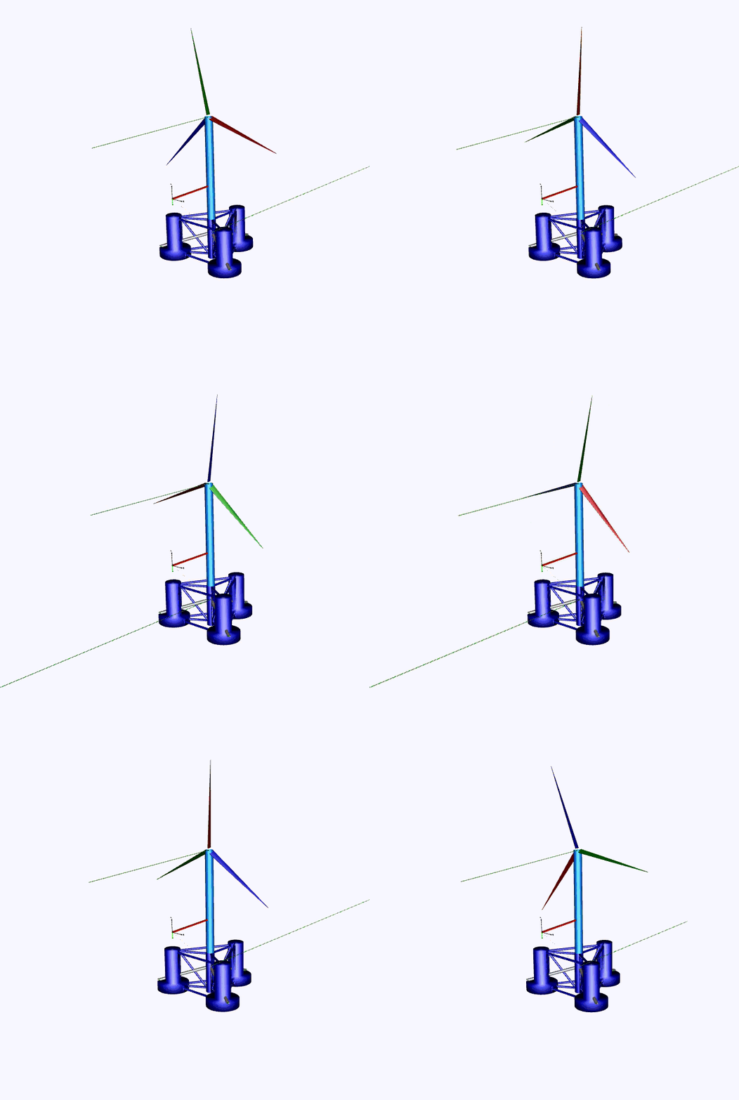
The platform in motion: OpenModelica’s native MultiBody animation, driven by the same model that produces every number in this post.

---

Part 1: Setting Up a Three-Line Floating Platform

We keep the same OC4 DeepCwind geometry from Part 1 and extend it to three mooring lines at 120° spacing: 200 m water depth, 837.6 m anchor radius, 40.868 m fairlead radius, giving each line a 796.732 m nominal horizontal fairlead-to-anchor offset (Part 1 used a single line at 785.7 m).

Line	Azimuth	Anchor (x, y, z)	Nominal horizontal offset
1	0°	(837.6, 0.0, -200.0) m	796.732 m
2	120°	(-418.8, 725.3, -200.0) m	796.732 m
3	240°	(-418.8, -725.3, -200.0) m	796.732 m

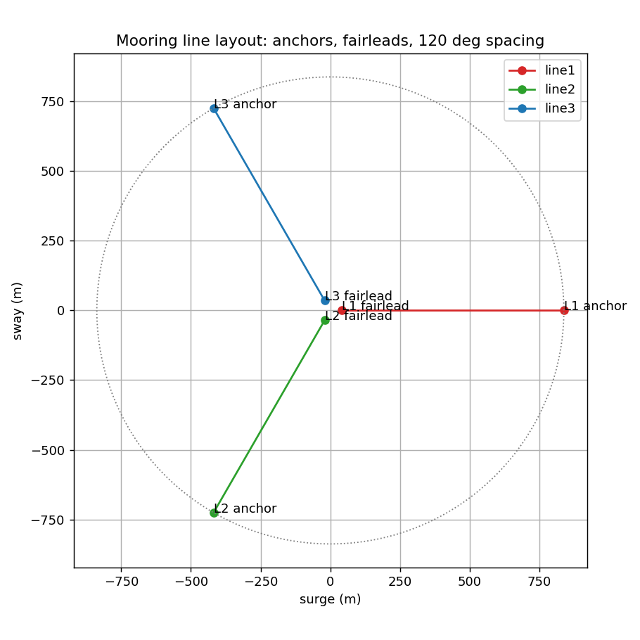
Plan view of the three-line layout: anchors, fairleads, and the nominal 796.7 m offset circle, all 120° apart. line_geometry.py derives the sway component as -sin(azimuth), matching Modelica’s own frame convention for mooringLineNRotation rather than the naive +sin(azimuth) a first pass might reach for.

We model the platform as a single rigid body riding on six stacked joints — three prismatic (surge along X, sway along Z, heave along Y), then three revolute (yaw about Y, roll about X, pitch about Z). Three of those six get a genuine hydrostatic restoring spring — heave, roll, and pitch — sized directly from the platform’s waterplane geometry:

DOF	Stiffness
Heave	3 757 kN/m
Roll	1.453×10⁶ kN·m/rad
Pitch	1.453×10⁶ kN·m/rad

Roll and pitch share the same value by the platform’s 3-fold symmetry, and both come entirely from the waterplane-pressure term, ρgI_waterplane. I_waterplane is the second moment of the waterplane area about the roll/pitch axis — for OC4’s one main column (3.25 m radius) plus three offset columns (6.0 m radius, 28.868 m off-centerline), that’s the parallel-axis sum:

I_waterplane = πr_main⁴/4 + 3(πr_offset⁴/4) + 3(πr_offset²)R_offset²/2 ≈ 144 518 m⁴

ρ_water g I_waterplane ≈ 1025 × 9.81 × 144 518 ≈ 1.453×10⁹ N·m/rad, which matches the reference OC4 HydroDyn input file’s roll/pitch coefficient (1.4513×10⁶ kN·m/rad) to within 0.1%. We deliberately leave the weight/buoyancy heeling moment out of that spring — world.g stays at its default value, so gravity acting on the platform, tower, and rotor-nacelle masses produces that moment directly, the way it would on a real hull. Folding it into the spring too would double-count it.

Heave’s 3 757 kN/m isn’t derived the same way: it’s the OC4-published ρ_water g A_waterplane constant, taken directly from the reference model rather than computed from the column geometry above.

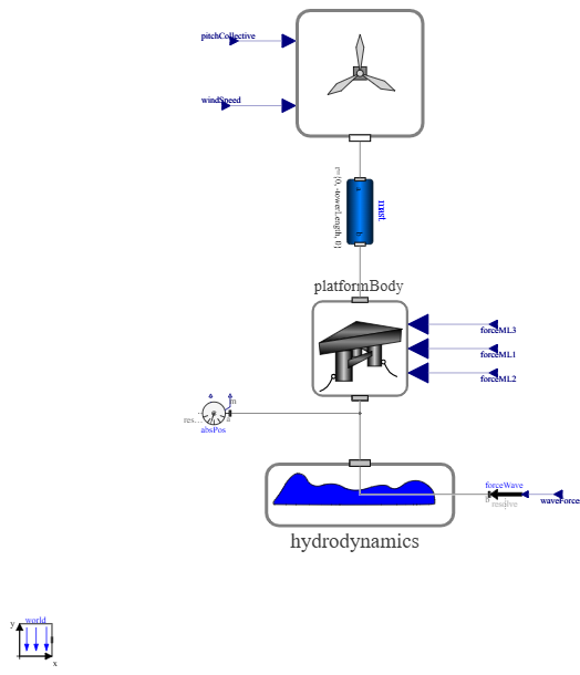
The top-level Modelica diagram for FOWT.mo — the bare model actually exported to FOWT.fmu. blades feeds thrust through mast into platformBody, which takes the three mooring line forces (forceML1/2/3) and hands off to hydrodynamics — the component carrying the surge/sway/heave/roll/pitch/yaw joints and the springs above. pitchCollective, windSpeed, and waveForces are raw external inputs with no internal tables — Python drives all three every step.

Rotor aerodynamics run in every simulation here — NREL 5-MW blade geometry with a simplified Ct·V² thrust formula, hub-height wind drawn from the same Kaimal turbulence time series as the sea state, and a closed-form collective-pitch control law holding thrust at its rated value once wind passes 11.4 m/s. Two sea states drive the loads in this post:

Sea state	Hs	Tp	Wind speed	Turbulence intensity
Operational	2.5 m	10 s	12 m/s	6%
Storm	6.0 m	14 s	20 m/s	12%

Wave elevation comes from a JONSWAP spectrum (environment/wave_model.py) and feeds environment/loads.py, which turns it into a surge force time series applied along the platform’s X axis. Wind speed feeds the FMU’s rotor directly, every step, driving real aerodynamic thrust through the control law above — this is wind and wave loading together, not a wave-only simplification.

---

Part 2: Building the Dynamic Co-Simulation Loop

The FOWT model — models/WindTurbines/Models/FOWT.mo — stacks six joints in sequence: surge, sway, heave, yaw, roll, pitch. Each translational DOF carries a spring-damper for hydrostatic and mooring stiffness; each rotational DOF carries its own spring-damper for pitch/roll righting moment, and a linear spring (bouyancyDamping) handles the heave waterplane stiffness specifically. Three fairlead frames, 120° apart, accept mooring line forces as forceML{1,2,3}[1..3] vector inputs; wave force enters separately as waveForces[1..3].

We export the whole thing as a single FMI 2.0 co-simulation FMU with omc (OpenModelica 1.24.4): models/FOWT.fmu, used for both sea states, since wind and wave are fed in as external inputs rather than baked into the model. From there, Python (simulation/cosim_runner.py, via FMPy’s FMU2Slave) steps the FMU at 0.001 s. 0.001 s is the largest step we found stable across a full 200 s run:

for i in range(1, n):
    platform_state = {key: series[key][i - 1] for key in MOTION_OUTPUT_NAMES}

    forces = []
    for line_index in range(3):
        fairlead = fairlead_world_position(platform_state, line_index)
        fx, fy, fz, tension = resolve_line_force(anchors[line_index], fairlead, mooring_model)
        forces.extend([fx, fy, fz])
        tensions[f"tension{line_index + 1}"][i] = tension

    fmu.setReal(mooring_input_vrs, forces)
    fmu.doStep(currentCommunicationPoint=t[i - 1], communicationStepSize=dt)

    values = fmu.getReal(motion_output_vrs)
    for key, value in zip(MOTION_OUTPUT_NAMES, values):
        series[key][i] = value

flowchart LR
    A["6DOF state, step i-1"] --> B["x3 lines: fairlead position"]
    B --> C["mooring model: force + tension"]
    C --> D["fmu.setReal: forceML1/2/3"]
    D --> E["fmu.doStep, dt = 0.001 s"]
    E --> F["fmu.getReal: 6DOF state, step i"]
    F -.next step.-> A

This is the feedback loop a static benchmark simply can’t exercise, and now three times over: each line’s mooring-model input on step i depends on the FMU’s full 6DOF output from step i-1, which itself depended on all three line forces from step i-2, and so on, all the way back.

---

Part 3: Two Mooring Models, One Interchangeable Interface

Both mooring models implement the same compute(horizontal_offset) -> dict interface, called once per line, three times per step:

• CatenaryMooring — Part 1’s Newton catenary solve, ground truth, run fresh every step. Caps at ~2190 kN at the 807.6 m taut limit.
• OnnxMooring — Part 1’s cached MLP surrogates, a forward pass instead of a solve. Clipped to the same taut cap so it never extrapolates past it.

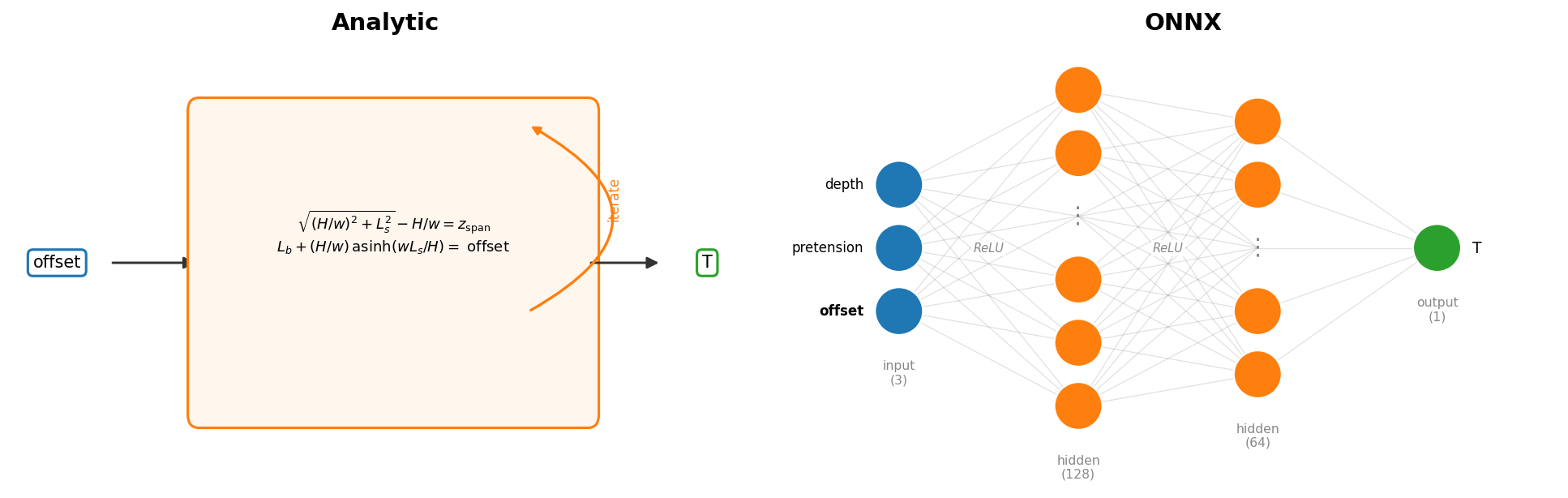
Same interface, different insides. CatenaryMooring (left) solves two nonlinear catenary equations for H and L_b fresh every call. OnnxMooring (right) skips the solve entirely: a small MLP with weights frozen at Part 1’s training run, one forward pass, no iteration. Swapping one for the other is a one-line change — run_cosim(CatenaryMooring(), ...) vs run_cosim(OnnxMooring(...), ...) — everything else in the loop stays identical.

That swap happens in the Python loop, not inside the .mo model. Wolfram System Modeler ships a built-in ONNX-import block, so the surrogate could sit inside the Modelica diagram there. OpenModelica 1.24.4 has no equivalent, so we push the boundary out to the FMU’s edge instead: FOWT.fmu only ever sees three force vectors over forceML{1,2,3}, and cosim_runner.py decides one level above whether those came from a Newton solve or an MLP. The FMU never needs to know which.

---

Part 4: Results in Both Sea States

Sea state	Hs	Tp	Wind speed	Turbulence intensity
Operational	2.5 m	10 s	12 m/s	6%
Storm	6.0 m	14 s	20 m/s	12%

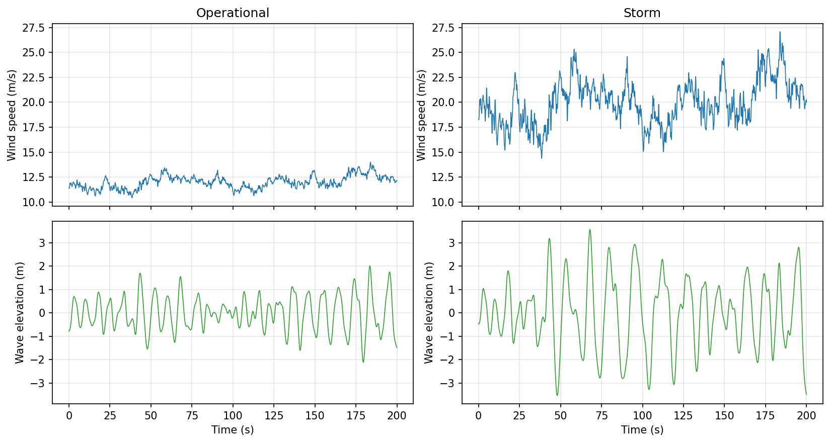
The Kaimal wind and JONSWAP wave time series actually driving the FMU each step, both sea states, full 200 s run.

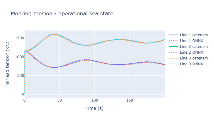
Operational sea state. Catenary (solid) against ONNX (dotted).

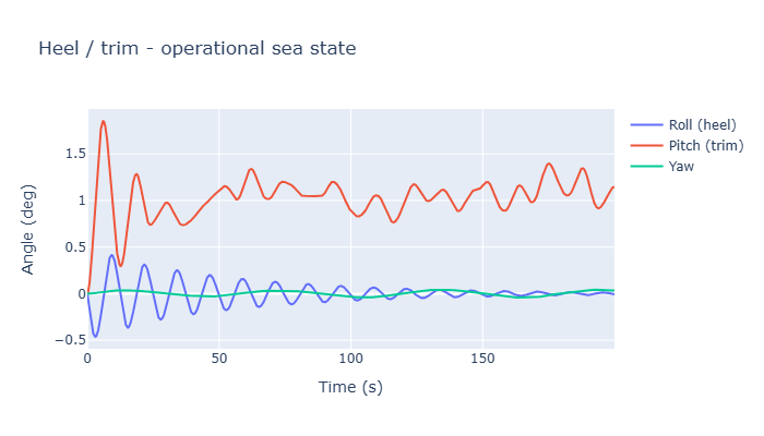
Heel, trim, and yaw, operational sea state.

Surge peaks at 13.8 m — thrust, not wave force, is the dominant driver here. Pitch (2.9°) confirms it: a wave-only run has no mechanism to sustain trim that large. All three lines stay well short of the 2190 kN taut cap.

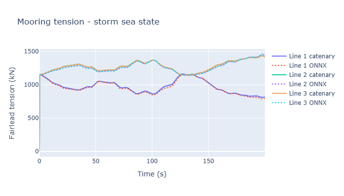
Storm sea state. Catenary (solid) against ONNX (dotted).

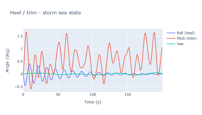
Heel, trim, and yaw, storm sea state.

Surge barely moves versus operational (13.78 m vs 13.77 m) despite 2.4× the wave height and wind well past rated speed — the collective-pitch control law caps thrust at rated value above 11.4 m/s, so storm-strength wind drives no more steady thrust than a calmer day at rated speed. Tension follows suit: every line’s range sits within a few kN of its operational counterpart.

Quantity	Operational	Storm
Surge, max abs	13.77 m	13.78 m
Heave, max abs (rel. to start)	0.89 m	0.89 m
Roll (heel), max abs	0.10°	0.25°
Pitch (trim), max abs	2.90°	4.03°
Yaw, max abs	0.05°	0.04°
Tension 1, range	731 – 1203 kN	731 – 1203 kN

Same compute(offset) swap, same loop, two sea states apart — the methodology doesn’t care which load case is driving it.

---

Part 5: So, What Did We Learn?

The headline: the same compute(offset) interface, the same co-simulation loop, ran end to end under two different mooring models and two different sea states without anyone touching FOWT.fmu. That’s the result this post set out to test — Part 1’s surrogate had only ever proven itself on a frozen platform, and a fully dynamic 6DOF loop is a different demand entirely.

Sea state	Runtime, catenary	Runtime, ONNX	Mean abs diff	Max abs diff
Operational	102.7 s	49.4 s	16.5 kN	49.2 kN
Storm	106.4 s	50.0 s	16.5 kN	46.5 kN

Both sea states land in the same range: mean diff ~16.5 kN, max 46-49 kN, against 1200-1700 kN tensions in play. Runtime tracks step count, not which mooring model is in the loop — three solves × 200,000 steps either way — so the gap between catenary and ONNX holds steady across both sea states.

One limitation worth carrying into Part 3 of this series: both mooring models are quasi-static. compute(offset) returns the equilibrium tension for a given offset, with no line mass, inertia, or added-mass dynamics of its own. Real chain has weight and drag that lag the platform’s motion — snap loads and line resonance a quasi-static catenary, or a surrogate trained on one, can’t produce by construction.

---

Code: vedat-s/Automation · part2_dynamic_mooring/